The specialized builtins are likely to be only rarely used, but can be very helpful when trying to accomplish certain things. These builtins operate on expressions. There are some specialized builtins that operate on arrays, and these are included in
. You'll find them helpful in setting up specific scenarios for a model simulation (COUNTER, CGROWTH, RUNCOUNT, SENSIRUNCOUNT), in doing simple trend analysis and extrapolation (FORCST, TREND), for simplifying computation in project models (REWORK), and in reusing or defining data sets for graphical functions (LOOKUP). Together, the miscellaneous functions offer a wealth of capabilities which can fill out the details of your model.
This section describes the following builtins:
In many instances, you'll want a stock to grow in compounding fashion, at a certain percentage rate per unit of time. You'd like to input the percentage growth rate, and to have the results of the process be independent of the DT that's being used in the model simulation.
The CGROWTH function enables you to define such DT-independent growth rates. Simply provide CGROWTH with a per-period percentage growth rate. When embedded in a compounding process, CGROWTH will ensure that the stock grows at the per-period rate you've specified, independent of the DT that's being used.
Example:
Growth Fraction = CGROWTH(10) produces 10% per unit time compound growth for the stock illustrated below. The specific numerical results of this compound growth process will be independent of the DT being used for the simulation.
Returns the current system clock time on the computer the software is running on. The time is the number of seconds since midnight, January 1, 1970 (often referred to as epoch time). Generally, this function is most useful for published simulations for which data are being collected. See Data Collection for more discussion and ways to convert this value to a recognizable date and time.
The COMBINATIONS builtin calculates the number of r-element subsets (or r-combinations) of an n-element set. The mathematical notation for this calculation is: n! /[r! * (n-r)!]
Example:
COMBINATIONS(5, 3) = (5 * 4 * 3 * 2 * 1) /[(3*2*1)*(2*1)] = 10
The FACTORIAL function calculates the factorial of n (traditionally noted as n!).
Example:
FACTORIAL(5) = 5 * 4 * 3 * 2 * 1 = 120
The LOOKUP builtin evaluates the <graphical variable> at the given <expression> (versus using the equation stored in the graphical function itself). This function uses the interpolation model (Continuous, Extrapolated or Discrete) specified in the graphical.
The LOOKUPAREA builtin returns the area under the <graphical variable> for all X values between <fromx> and <tox>. For example, a graphical that is constant at 1 will have an area given by the <tox>-<fromx>. This is a convenient function for normalizing the output of graphical.
If <fromx> is omitted, the computation will be made from the beginning of the graphical. If both <fromx> and <tox> are omitted the computation will be made over the entire graphical. You can change the order of <fromx> and <tox) - so that LOOKUPAREA(var,3,5) is the same as LOOKUPAREA(var,5,3).
For continuous and stepwise graphicals LOOKUPAREA will ignore (effectively treat as 0) values below the minimum X value of the graphical or above the maximum X value.
For extrapolated graphicals the area is computed using the extrapolated value.
The LOOKUPINV builtin reverses the normal lookup logic returning the x value in the <graphical variable> that would generate the given <expression> as output. As long as the graphical is monotonic (the y value getting bigger for each successive x value, or the y value getting smaller for each successive x value) it will return a value. If the graphical is marked as Extrapolated it will use extrapolation to compute a value, otherwise it will return the first or last point when out of range.
If a graphical is not monotonic (including starting of stopping with a flat spot), the first x value to generate the y value will be returned. If there y value is out of range then NAN will be returned.
These LOOKUP builtins (along with LOOKUPAREA above), allow you to get information about the values in a graphical function. LOOKUPMIN and LOOKUPMAX find the minimum and maximum Y values in a graphical. LOOKUPMEAN is different in that it finds the mean X value treating the Y values as probabilities (to find the mean Y values use LOOKUPEA(var,x1,x2)/(x2-x1). All take the same arguments.
<graphical variable> is a variable that is a graphical. If the variable is not a graphical these builtins will all return NAN. If the graphical values are being controlled via import, a change from the Results Panela, or a Graphical Input Device on the interface the newly set graphical will be used. If it is being controlled at a constant value (for example via a slider), the original graphical will be used. If this argument is used by itself then the full range of the X axis will be used.
<tox> is the last value of X to consider. If there is no value for <fromx> the first X value in the graphical will be used.
<fromx> is the first value of X to consider.
Note The values of <tox> and <fromx> can be provided in either order. So that LOOKUPMAX(var,1,7) and LOOKUPMAX(var,7,1) return the same value.
LOOKUPMEAN is a specialized builtin that will normally be called with only a single argument. It treats the graphical values between <fromx> and <tox> as describing a probability density function (pdf) and computes what amounts to the expected value of X given that pdf. This can be very useful when working with LOOKUPRANDOM, and adjusting the delay time for a conveyor using a profile as described in Spreading Conveyor Inputs.
Most commonly, LOOKUPMEAN will be used on a distribution with the x axis ranging from 0 to 1. For example, to determine the appropriate transit time for a conveyor to achieve a desired average delay you would use:
delay_profile ((0,0),(0.5,1),(0.8,0.01),(0.1,0))
average_delay = 8
transit_time=INIT(average_delay/LOOKUPMEAN(delay_profile)
The conveyor would then use transit_time as the transit time, and the inflow would use delay_profile as the profile.
Note The above equations require that the graphical be defined on the range 0 to 1, otherwise the max value will be distorted and the mean transit time through the conveyor will not be average_delay. Alternatively, using INIT(average_delay/(LOOKUPMEAN(delay_profile)-x_min)/(x_max-x_min)) would work
The GAMMALN builtin returns the natural log of the GAMMA function, given input n. The GAMMA function is a continuous version of the FACTORIAL builtin, with GAMMA(n) the same as FACTORIAL(n-1). Because this builtin returns the log of the result, it's possible to call it with larger arguments than FACTORIAL. This makes it very useful for computing ratios of different factorials. For example, EXP(GAMMALN(1001) - GAMMALN(951) - GAMMALN(51)) is the same as COMBINATIONS(1000,50).
The INVNORM builtin calculates the inverse of the NORMALCDF builtin .
The LOOPSCORE builtin returns the relative contribution of a loop to determining behavior at each time in the simulation. See Loops That MatterTM Overview for discussion and references.
The arguments <var1>, <var2> and so on must define a feedback loop. If they do not, LOOPSCORE will return NAN at all times.
LOOPSCORE is added automatically when you create Loop variable from the Loops Panel. Typically, this is the only way it is used, so you won't ever add it by hand. Like a Summing Converter, a Loop Score variable does not have any connectors going in. Unlike a Summing Converter, however, you can't use a Loop Score variable in the equation of another variable. This is because Loops Scores are not computed until after a simulation finishes, and thus the value returns is always NAN during the simulation. For this reason the variable will also not animate on a graph during simulation, but only display afterward.
You can change a Loop Score variable to a Pathway Score variable. This will change the LOOPSCORE builtin to the PATHSCORE builtin, and also add the first <var> at the end to close the path.
The PERCENT builtin gives the value of fraction, expressed as a percentage. The fraction value can be either a variable or a constant.
Examples:
PERCENT(.65) equals 65
PERCENT(1.22) equals 122
The NORMALCDF builtin calculates the cumulative Normal distribution function between the specified z-scores, or, when the mean and stddev (standard deviation) are given, between two data values. The cumulative distribution function integrates (sums) all values of the Normal probability distribution function between the left and right endpoints. To sum from negative infinity, use a z-score of -99. To sum to positive infinity, use a z-score of 99.
The following graph shows the behavior of the NORMALCDF function for -4 = z = 4.
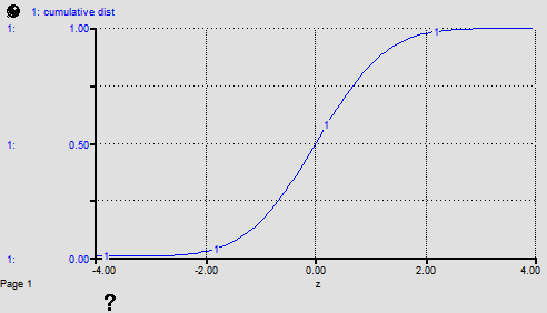
The equation NORMALCDF(-99, TIME) was used to make this graph. Note that the NORMALCDF very closely approximates the logistic function, or S-shaped growth. It can be used to formulate, using an equation, several types of common graphical functions:
Note: A z-score can be calculated with the formula: (data_value - mean)/stddev.
The PATHSCORE builtin returns the product of the raw (unnormalized) Link Scores along a path of connected variables. See Loops That MatterTM Overview for discussion and references.
The arguments <var1>, <var2> and so on must be on a path (that is <var1> must be a cause of <var2> and so on. If are not, PATHSCORE will return NAN at all times.
When PATHSCORE is called with two variables it returns link score. While PATHSCORE can be used in any equation, it will be automatically input into the equation for a Pathway Score variable. You can create a Pathway Score variable from a Loop Score variable by changing its type. This sill add the first entry last in order to close the loop. You can also create a Loop Score variable from a Pathway Score variable - this will remove that last variable since the Loops assumes closure.
The PERMUTATIONS builtin calculates the number of permutations of an n-element set with r-element subsets. The mathematical notation for this calculation is: n!/(n-r)!
Example:
PERMUTATIONS(5,3)=5*4*3*2*1/2*1=60
In many instances, you'll want to represent a rework process. In the following figure, for example, a production process is used to draw down a work backlog. A portion of the work (defectives) is shunted back to an earlier stage in the process to be reworked.
In the following figure, a conveyor represents an inspection activity. The leakage flow from the activity moves rejected material to an earlier stage in the process, where it will subsequently be re-worked.
In either situation, using a simple fraction to represent the rework percentage will overstate the cumulative flow of material through the rework process. Each time that material passes through the inspection activity or production process, a fraction of it will be sent back to be re-worked. Double-counting can ensue. For example, if 100 units are sent through the process initially, a 10% defective fraction would send 10 units back to be re-worked in the first round. In the second round, 1 unit (10% of the 10 units) would be sent back. And so on. After the fact, more material than 10% has been re-worked! In most cases, this isn't what you intended.
To get around this double-counting phenomenon, the software provides the REWORK builtin. Use it only to represent a rework flow which deposits material at a point somewhere upstream in the main chain. Simply specify the percentage of total work flow that you want to flow back upstream to be reworked. The percentage value should be a value between 0 and 100.
Notes: When using a draining process to represent
the rework flow, the REWORK builtin is not an appropriate choice.
When the defective flow goes to a cloud, double-counting is not an issue.
Hence, REWORK isn't required.
Example:
The previous figure shows the results of using REWORK(10) to define the leakage fraction for the leakage flow from "Inspection Activity". With a total of 100 units of material entering the system through the "entering wip" flow, a total of 10 units of work flow through the "failing inspection" flow, over the course of the simulation.
Returns the current version of the software. The version is in the form major.2digitminor2digitrevision (e.g. 3.0501 for version 3.5.1) so that it will be increasing with increasing version number even when the minor version or revision is larger than 9 (thus it will be 3.1114 for 3.11.14)
Use this builtin to detect software versions that may not work with your model. For example
IF SOFTWAREVERSION < 3.05 THEN 1/0 ELSE 0
will cause a divide by zero in software prior to version 3.5. You can put information in the documentation as to why this is done. Alternatively, you could set up a message from Simulation Events.
The SYSTEMCHANGE builtin returns the system change metric that is reported in the Loops Panel. See Loops That MatterTM Overview for discussion and references.
The optional argument specifies the loopset (each loopset has a different system change). If loopset 1 is used. If you specify a loopset that does not exist NAN is returned. NAN is also returned during the simulation, as this result is only finished after the simulation has completed, and the loop scores have been computed.
SYSTEMCHANGE must appear alone in the equation, it can't be part of an expression.