Array Operation builtins
Array Operation builtins operate on arrays with additional expressions. Many operate on two or more arrays with the expectation that the wildcard (*) positions on the different arrays will align. These functions work on array ranges, and there is in-depth discussion of this in Specialized Array Manipulation.
Note Not all of the builtin functions can be used in Array expressions. You can't use any builtin that has a value depending on previous results (this includes the Delay builtins, Data builtins
and Random builtins ). You also can't use any other array or array operation builtins in the expression (it is not possible to nest array builtins.)
Note Array operations require variables as inputs in at least one position. Unlike the Array builtins
it is not possible to use an expression with wildcards.
This section describes the following builtins:
ALLOCATE(<available>, <index>, <target_array>, <priority_array>, <priority_spread>, [<shape>])
The ALLOCATE builtin determines a vector of quantities that can be used to distribute available across the different values of index. This is done based on a target for all indices specified in target_array with priorities (or attractiveness) specified in priority_array. It available is sufficient to satisfy the sum across target_array then the target value at index is returned. If available is not sufficient, a portion of it is provided based on the associated element in priority_array relative to the other elements. The argument priority_spread is used to determine whether portions of lower priority requests are supplied before all of higher priority requests are supplied. The optional shape argument determines the extent of that spreading.
If priority_spread is 0 then higher priority indices are supplied first. When it is positive higher priority indices will get a larger share or their target, but lower priority indices may also receive a portion of their target. shape determines the nature of this spread. The default 1 uses a rectangular spread, 2 a triangular spread (less sharing), 3 a normally distributed spread (more sharing), and 3 an exponentially distributed spread (even more sharing). It is useful to experiment with priority_spread and shape to get the desired allocation outcomes.
Both target_array and priority_array must be array slices of the same size across the values index takes on. available, priority_spread and shape can be any expression, but can not vary by index.
Examples:
ALLOCATE(candy_available,kid,appetite[*],weight[*],0) would share the candy among the kids with the heaviest kids getting the candy first, then the lighter kids. Both appetite and weight are arrayed by kid.
ALLOCATE(demand[product], producer, capacity[product,*], attractiveness[product,*], 2) would allocate product demand (by product) to different producers based on their capacity and attractiveness for that product. The 2 argument means that producers having attractiveness for the product within 2 of other producers will potentially sharing in that allocation.
ALLOCATE(funding,state,need[*],poverty_index[*],10,3) would allocate funding to different states based on their need (which would likely be proportional to population) with higher priority given to states with a higher poverty_index. Using a shape of 3 and a big spread means that people from all states would get something.
Note It is important that available, priority_spread and shape take on the same the same value for all entries in index (stated another way, these values should not be arrayed by index). Otherwise too much may be allocated or not all of the available amount used and some targets left unsatisfied.
Note The units of the first and third arguments should match, and will be the units returned. The units of the fourth and fifth arguments should match, and shape should be dimensionless.
INTERPOLATE(<arrayed variable>, <val1> [<val2>,...])
The INTERPOLATE builtin calculates the interpolated value of an N-dimensional set of points based on inputs computed on the unit interval [0,1]. It can be used to provide a continuous lookup mechanism for values that pass through all of the specified points. In 1 dimension this is the same as the behavior of a graphical function based on a vector of values.
The first argument must be an arrayed variable or a subset (slice) of an arrayed variable. For example, if there is a three dimensional array called points, then you could specify points directly with 3 additional arguments, or points[2,*,*] with 2 additional arguments.
The arguments should be normalized so they provide a value between 0 and 1. If the value is less than 0, the first entry in the associated dimension will be used. If the value is above 1, the last entry will be used. Between values the weighted average of the entry before the one associated with the input and the one after will be used. For example, if there are 5 entries, then a value of 0.3 would be between the second entry (at 0.25) and the third entry (at 0.5) and 80% of the value of the second entry and 20% of the value of the third would be used.
There must be at least 2 elements in each dimension of the arrayed variable, but there is no limited to how many there are beyond that, and no requirement that the different dimensions have the same number of entries. In all cases, the entries will be divided into an equal number of regions (n-1 internal and 2 external) and the results based on that.
Examples:
If pts[Dim1] is 0,2,4, then INTERPOLATE(pts, 0.75) would return 3.
If pts2d[Dim1,Dim2] is (0,2,4),(8,6,5) then INTERPOLATE(pts2d, 0.75, 0.25) would return 5.5. You can think of this as taking 25% of (0,2,4) and 75% of (8,6,5) to get (6,5, 4) and then taking the halfway point between 6 and 5 to get 5.5. Alternatively, since the 0.25 position of 3 numbers is half way between the first two, it works to take the halfway points between 0 and 1 (1) and that between 8 and 6 (7) then take 25% of 1 and 75% of 7 to get 22/4 or 5.5.
MATRIXINVERT(<matrix> , <row>, <column>)
The MATRIXINVERT builtin returns the indicated row and column entry for the inverse of matrix. It will almost always be called in the form
MATRIXINVERT(mymatrix[*,*],@1,@2)
or
MATRIXINVERT(mymatrix2[otherdim,*,*],@2,@3]
where mymatrix is a square 2 dimensional array, and mymatrix2 is a 3 dimensional array. In both cases it is a square 2 dimensional matrix that is being inverted. In the first case the [*,*] is optional.
Matrix inversion can be useful for certain specialized computations such as those used in Input/Output analysis. There is a sample model demonstrating this here.
MLPANN(<input> , <shapes>, <weights>, <biases>, <activation type>)
The MLPANN builtin allows you to create a Multi-Layer Perceptron Artificial Neural Net. This is useful for approximating functional relationships using trained neural nets, where the training is done using the optimizer.
<input> is a vector of inputs to be passed through the neural net.
<shapes> is a vector of values that describes the topology of the neural net. The number of elements in it determines the number of layers in the network, and the value of each element the number of nodes in each layer.
<weights> is a vector of values that specifies the weight to be given to the incoming connection to each node (on all layers). The total number of weights must be equal to the product of the elements of the <shapes> vector. The weights are typically included as part of an optimization to train the neural net.
<biases> is a vector of values that scale the input to each of the nodes. It can be a vector of 1s, but must have the same number of elements as <weights>.
<activation_type> specified the type of activation function used. A value of 1 will use a tanh activation function (most common), 2 a sigmoid activation function, and 3 a non-negative activation function (negative values treated as 0) function. Any other value will use a linear activation function (no attenuation).
PERCENTILE(<arrayed variable>, <cut>[,<lower cut>, <volume variable])
The PERCENTILE builtin calculates the value across an array slice that is reached the percent of the time specified by cut. For example if cut is 25 then 25% of all elements of the array slice will be below the value returned (and 75% above). If tlower cut is specificed then the value returned is the same as
PERCENTILE(array_slice,cut)-PERCENTILE(array_slice,lower_cut)
This is done to make it simply to use the output of PERCENTILE with an Area Graph where the different series build up from the min (0 cut) to the max (100 cut). If both cut and lower_cut are 0 then the minimum will be returned, otherwise cut must be greater than lower_cut or 0 will be returned.
Examples:
Median Salary for Employees = PERCENTILE(Salaries,50)
Maximum Salary for Employees in Boston = PERCENTILE(Salaries[Boston,*],100)
Minimum Salary for Labor Groups 1 to 3 = PERCENTILE(Salaries[*,1:3],0)
Difference between min and median for employees in Boston = PERCENTILE(Salaries[Boston,*],50,0)
When the optional fourth argument volume variable is used, the first argument is treated as an attribute, and the second as a volume. The return is then the attribute value which cut percent of the total volume is below. When this argument is used, and lower cut is 0, the value returned will be the percentile of the attribute, not the different with the value of the smallest attribute (which may be bigger than 0).
Example - both Population and Cohort_Avg_Age are arrayed by Sex,AgeCohort:
Median_Age[Sex] = PERCENTILE(Cohort_Avg_Age[Sex,*],50,0,Population[Sex,*])
Composite_Median_Age = PERCENTILE(Cohort_Avg_Age,50,0,Population)
Note With 5 year cohorts Cohort_Avg_Age would be 2.5, 7.5, 12.5...
Note PERCENTILE with 4 arguments will never return less than the first element of the first argument or more than the last, though in between it will interpolate between array element values.
Note When used with a fourth argument lower cut will almost always be 0.
RANK(<arrayed variable>, <rank number>, [<secondary sort array>])
The RANK builtin gives the numerical index of the arrayed variable with the given rank number when the array is sorted in ascending order. The optional secondary sort array specifies the secondary sort field for variables with the same value. The secondary sort array must be the same size as the arrayed variable, or the secondary sort won't occur (this is only enforced when you simulate the model, so you won't be warned).
Example:
If array A contains the values { 6, 2, 8, 5 }
RANK(A, 2) will equal 4 (i.e., the fourth element of array A is the second smallest value)
Using RANK causes the specified array to be sorted once each time step (DT). For multi-dimensional arrays, you can pass one or more dimensions of the array to return the rank of a subset of the array.
Example:
Rank(Salaries[Boston,*],2) returns the rank of the second smallest salary in Boston.
To invert the RANK operation when it operates over all elements of a dimension you can use:
SUM(IF Ranking[*] = dimension THEN IDENTITY[*] ELSE 0)
Where IDENTITY[dimension] is defined by the equation
INIT(dimension)
This can be helpful if you want to restore the original order after operating on a sorted set of variables.
SHORTESTPATH(<adjacency>, <index>, <start>, <finish>)
The SHORTESTPATH builtin determines a vector of indices that represent the most efficient way to get from start to finish given the adjacency matrix. The adjacency matrix is a square matrix that represents the distance, time, or cost needed to get from one position in an array to another. It can be symmetric (so that getting from the 3rd to 5th positions has the same entry as getting from the 5th to 3rd) but will not always be. It can be arrayed by the same thing twice (as in distance[location,location] )or by two different things (as in travel_time[from,to]) so long as both array dimensions have the same size.
index is the index in the path being returned, with the first index always equal to start unless there is no viable path from start to finish in which case it will be NAN. start is the first place to visit from, and finish is the final location. The resulting path will have positive entries representing the sequence of entries to visit possibly followed by 0s if the path is shorter than the number of array elements (for example the shortest path from 1 to 2 might just be directly going from 1 to 2 even when there are 5 different locations).
If there is a NAN in adjacency it means it is not possible to get directly between two positions. In this case there may not be a path between locations and the SHORTESTPATH will return NAN for every index. Using a large number will guarantee that a path exists, though it might be very inefficient.
Normally all entries in adjacency will be positive numbers, except the diagonal entries which are usually 0 (and ignored in any case). If you do use negative values they are treated as relative to ensure convergence.
Examples:
adjacency
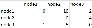
SHORTESTPATH(adjacency[*,*],node,1,2) would return 1,3,2 for the 3 different values of node.
SHORTESTPATH(adjacency[*,*],node,2,3) would return 2,3,0 for the 3 different values of node.
SHORTESTPATH(adjacency[*,*],node,2,1) would return 2,1,0 for the 3 different values of node.
Note It is important that adjaceny, start and finish be the same for all values of index. Otherwise the path will not be a coherent path.
Note adjacency needs to be a 2 dimensional square array at least 3x3 in size.
Note Paths are basically array indices and would typically be marked as Dimensionless.
TRAVERSALCOST(<adjacency>, <path>)
The TRAVERSALCOST builtin determines the cost of following path through adjacency. Typically, path will be values returned from SHORTESTPATH, but it can be any set of values indicating array elements.
The units of measure for TREVERSALCOST will be the same as those for adjacency. If this is measured in distance it is the distance traveled, time the time traveled and so on. Cost here, is being used in the general sense of burden.
Examples:
adjacency
If path is 1,3,2 then TRAVERSALCOST(adjacency[*,*],path[*]) would return7.
If path is 1,2,0 then TRAVERSALCOST(adjacency[*,*],path[*]) would return 10.
If path is 2,1,0 then TRAVERSALCOST(adjacency[*,*],path[*]) would return1.
Noteadjacency has to be a 2 dimensional n by n array and path needs to be a 1 dimensional array of length n.
 See Also