Data builtins report the value of model variables at a particular time in the simulation.
This section describes the following builtins:
The DERIVN builtin calculates the nth-order time derivative of input. The input value can be either a variable or a constant, but order must be a non-negative integer. The software uses a recursive finite difference technique to calculate time derivatives. The basic equation used in the calculation is:
dx/dt = (xt - x(t-dt))/dt
where t is current simulation time, and dt is DT, the simulation solution interval.
Because the DERIVN builtin uses previous values of input for its calculations, the builtin returns an initial value of 0.
Calculus cognoscenti will note that it's possible to use the chain rule to calculate dy/dx, where yand x are time-dependent model variables. Use this formula:
dy/dx = dy/dt ÷ dx/dt
Examples:
DERIVN(TIME,0) equals TIME (the zeroth-order derivative)
DERIVN(TIME,1) equals 1 (the first-order derivative)
DERIVN(SIN(TIME),4) calculates the fourth-order derivative of a sin function on time, which is equal to the sin function (except for the first 4 dts when DERIVN will return 0).
When the order argument to DERIVN is a number rather than an expression the units returned for the function are the units of the input divided by the units of time raised to the appropriate power. That is, the first derivative is per time units, the second per time units squared and so on. If the order argument is an expression, including just a variable, the units returned are the same that a number would return.
The ENDVAL builtin returns the ending value of input, from the most recent simulation run in a session with a model. You can use any expression for input, though it will typically just be a model variable or SELF. The first time you run the model after opening it, ENDVAL will return the initial value you've specified. If you don't specify an initial value, ENDVAL will return the initial value of input during the first run.
Example:
Is_Performance_Improving = Current_Performance_Indicator -
ENDVAL(Current_Performance_Indicator,0)This will look at the current performance, relative to the ending value of performance in the last simulation run of a given simulation session. In so doing, ENDVAL provides a mechanism for looking at run-to-run performance changes, and thus can provide a vehicle for triggering "as-needed" coaching to the model consumer.
You can use ENDVAL(SELF,init_val) to capture the value of a variable at the end of the previous run. This can be used to implement a custom version of RUNCOUNT as in:
My_RUNCOUNT = IF reset <> 0 THEN 0 ELSE ENDVAL(SELF,-1) + 1
Note You must include an explicit initial value when using SELF.
When you're editing a model, the ENDVAL function will reset (return the initial value) when you make changes to the equation using it directly, or through actions such as changing array definitions. In this case, it will act as if there is no previous run in the session.
Note Publishing a model from the interface will also cause ENDVAL to reset.
The FORCST builtin performs simple trend extrapolation. FORCST calculates the trend in input, based upon the value of input, the first order exponential average of input, and the averaging time. (Think of the averaging time as the time over which you want to calculate a trend.) Then FORCST extrapolates the trend into the future; you specify the distance into the future, by providing a value for horizon. If you don't specify an initial value initial, FORCST substitutes 0 for the initial value of the trend in input.
The FORCST builtin is equivalent to the structural diagram and equations shown in the following figure.
Example:
Sales_Forecast = FORCST(Sales,10,15,0) produces a forecast of sales 15 time units into the future. The forecast is based on current sales, and the trend in sales over the last 10 time units. The initial growth trend in sales is set to 0.
Tip: If you encounter noise in the variable to be forecasted, you may wish to filter the randomness by basing your forecast on an exponential smooth of the variable. To do this, use the SMTH1 or the SMTH3 function (described later in this section).
The HISTORY builtin returns the value of a variable at a prior time in the current run, or in another run (from the model or imported). <variable> is a model variable (or expression if called with 2 arguments) and <time> the time at which to get the value. If <time> is greater than the current time, or less than the first time available, HISTORY returns 0 unless the optional <run> parameter is used.
If the options argument <run> is used then HISTORY returns the value of the variable from another run. 0 is the current run (so that HISTORY(var,t,0) is the same as HISTORY(var,t)), 1 is the first active run as shown by the Data Manager, 2 the second and so on. Negative numbers can be used for the previous run as discussed below.
The <source> argument determines which run list to use. 0 is the active run list. 1 is the saved run list as shown in the Data Manager and -1 changes the meaning of <run> to be relative to the current run, so that 1 is the previous, 2 the run prior to that and so on. Alternatively, you can pass a negative value for <run> and leave <source> off to get this result.
If the <run> and <source> values specified do not identify a valid run HISTORY will return NAN. You can use the ISNAN builtin to check this. If <time> is before the start of the identified run the first value from the identified run is used, is after the last value.
By default, HISTORY will interpolate data. You can, however, specify that it return NAN except when time is within DT/2 of actual data points (this is the same logic as the Raw option discussed in Import Data dialog box. To do this use a decimal value of .5 in the <source> argument. For example HISTORY(population,TIME,1,0.5) would get the population points that exist in the first run, and return NAN at all other times.
Note The <run> and <source> parameters are evaluated only during initialization. If their values change during a run it will have no effect.
Note The first argument can be an expression when called with 2 arguments, but not when called with 3 or 4 arguments.
Note: HISTORY (stock, TIME-1) is the same as DELAY (stock,1) except at the initial time.
The INIT builtin takes the initial value of the stock, flow, converter, or expression, where the initial value for the variable has been calculated at the outset of a simulation.
Examples:
Distance_Traveled = Position - INIT(Position)
Computes Distance Traveled as the difference between current position and the initial value of position.
Debt_Ratio = Debt/INIT(Debt)
Computes Debt Ratio as the ratio of Debt to its initial value. When creating graphical functions, it's often useful to normalize the input to the graphical function in this manner.
These functions return results from a variable over a time range in the current run, or in another run (from the model or imported). RUNCUM the cumulative value, RUNMAX the maximum value, RUNMEAN the mean value and RUNMIN the minimum value.
<variable> is a model variable. If called with this as a single argument values from the run so far (including the current time) will be reported. For example
RUNMAX(sales)
will report the maximum value of sales in the run so far.
<fromtime> and <totime> specify the time range over which the maximum will be taken. If either of these is before the beginning of the run the computation will start at the beginning of the run. If after the end of a run for historic runs the computation will stop at the end of the run. If <fromtime> is greater than <totime> NAN will be returned. If <totime> is after the current time for the current run, then NaN will be returned unless the variable has imported time varying values in which case those values will be treated as an external run.
<run> specifies the run to draw the values from. Use 0 for the current run (the default), 1 is the first active run as shown by the Data Manager, 2 the second and so on. Negative numbers can be used for the previous run as discussed below.
<source>specified which run list to use when interpreting run. 0 is the active run list and is the default. 1 is the saved run list as shown in the Data Manager and -1 changes the meaning of <run> to be relative to the current run, so that 1 is the previous, 2 the run prior to that and so on. Alternatively, you can pass a negative value for <run> and leave <source> off to get this result for earlier runs.
If the <run> and <source> values specified do not identify a valid run NaN will be returned. You can use the ISNAN builtin to check this.
Examples:
RUNMEAN(infections,time-6,time) returns the 7 day moving average of infections including today's value.
Note Using 7 in the above would include both today and the same week day of last week - effectively the 8 day moving averate.
RUNCUM(cash_flow) returns the cumulative cash flow including the current period.
Note The above is the same as adding a stock with an inflow equal to cash_flow and then adding cash_flow*dt before reporting the value. RUNCUM(cash_flow, STARTTIME, TIME-DT) would return the stock value.
The PREVIOUS builtin returns the value of a variable or array at the previous time in the simulation. When there's no previous time, it returns the <initial> value.
Examples:
PREVIOUS(A, 0) returns the value of A at the previous time, or returns 0 if there's no previous time.
PREVIOUS(SELF,2) returns the value of the current variable at the previous time, or returns 2 if there's no previous time.
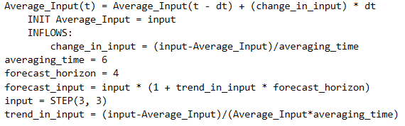
The TREND builtin calculates the trend in input, based on the value of input, the first order exponential average of input, and the exponential averaging time averaging time. TREND is expressed as the fractional change in input per unit time. If you don't specify an initial value initial, TREND substitutes the value 0 for the initial value of the trend.
The TREND builtin is equivalent to the structural diagram and equations shown in the following figure.
Example:
Yearly_Change_in_GNP = TREND(GNP,1,.04)
This equation calculates the annual change in the input GNP. It starts with an initial value of .04 (4% per year).