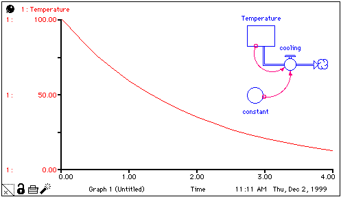
Consider the plot and model structure shown below.

The plot shows the idealized behavior of a real-world system; in this case, the temperature of a cooling cup of coffee. The model is idealized as well; if it were solved analytically, it would yield exactly the behavior exhibited by the plot.
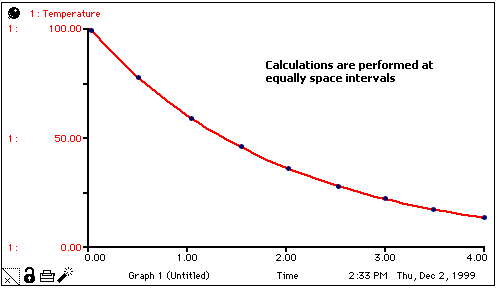
When the computer is used to simulate systems such as this, it's not possible to get an exact solution. Instead, a set of discrete calculations (the only kind that digital computers are capable of producing) is used to approximate the idealized curve. The software divides the time axis into equally-spaced intervals, each with a width of DT (or "delta time"). In this case, calculations are performed at discrete intervals, as indicated in the following graph.

In Stella, the equation structure that underlies the model diagram is of vital importance. The equations created behind the scenes as you hook together stocks and flows are known as "Finite Difference Equations." For example, on the Equation layer for the cooling model, there would be a set of equations that look like these:
Temperature(t) = Temperature(t-dt) + (-Cooling)*dt
INIT Temperature = 100
Cooling = Temperature * Constant
Constant = 0.5
In a model, each stock equation (in this case, the equation for Temperature) is a finite difference equation. Conceptually, solving finite difference equations is straightforward. It involves a two step initialization phase, and a three step iterative evaluation phase:
Step 1. Create a list of all stocks, and any flows or converters required to initialize those stocks, in the order of evaluation based on their equation. If a flow or converter has an initial equation that equation is used to determine the evaluation order.
Step 2. Calculate initial values for all stocks. Any flows or converters required to do this will also be computed (using their initial equations if they have them).
Step 3. Create a list of all flows and converters in the order of evaluation using their active equations.
Step 4. Calculate the values of all flows and converters based on the initial values of the stocks.
Before you simulate a model these steps are carried out in the background and the resulting values are available for display. Every time you make a change to the model these steps are repeated in the background.
Step 1. Use values of stocks (from the previous phase or Step 2) to calculate new values for flows and converters.
Step 2. Estimate the change in stocks over the interval DT (simply multiply flows by DT for Euler integration, other methods are more complicated). Calculate new values for stocks based on this estimate.
Step 3. Update simulation time by an increment of DT. Stop iterating when Time >= simulation To Time.
Step 2 of the iteration phase is a critical one: How does one estimate the change in the value of stocks over the interval DT? The software provides different algorithms for doing this estimation: Euler's method, 2nd-order Runge-Kutta, and 4th-order Runge-Kutta method.
You select the method your model will use in the Model Settings Properties panel box.
When you pause a model it stops after step 1 of the iteration phase. The values of all stocks, and the values of flows and converters based on those stocks will have been computed, but the stocks are and time will not be updated. When the model is resumed, step 1 is repeated and then step 2 and 3.
Because step 1 is repeated, there may be different values computed for the flows and converters the second time it is executed. This can result when a model constant is changed while the model is paused.
When working on the model window, step 1 is repeated each time a change to a constant is made. All values displayed on the model, including numeric displays, graphs, tables, and tooltips, will reflect the new computation. This means that if you pause a simulation and change a constant, you may see graphs and tables updating based on the new constant value you have set.
Although pausing works the same way on the interface, what is displayed are the values from the previous DT (more precisely the previous Save Interval computations) for flows and converters. For specific controls, you can optionally ask to see (or use) the current results. Because these results change every time an input is changed (for example by the user moving a slider) the output will change in response to use input even thought time is not changing.
The option to display the values of flows and converters that will be computed is available for Animation Object(Interface), Gauge(Interface), Numeric Display Properties, Spatial Map(Interface), Status Indicator(Interface), and Button (Interface)for conditional computations.
For additional discussion on pausing see Initialization and Pausing