The test input builtins enable you to conduct controlled experiments on your model. Typically, a PULSE, RAMP, or STEP is appended to an inflow or outflow equation. When the builtin is activated (at the time you specify), it will knock the system out of its previous state. You can then observe how your model responds to this idealized test.
Conducting controlled experiments using idealized inputs such as PULSE, RAMP, and STEP is an excellent way to build understanding of the inner workings of your model.
This section describes the following builtins:
The COSWAVE builtin returns a time-dependent cosine wave, with the specified amplitude and period. To generate the cosine wave, the COSWAVE builtin uses the absolute value of the amplitude you specify. To produce meaningful wave results, choose a DT that's significantly smaller than the period of the wave. A DT equal to a quarter of the period gives triangle waves. A smaller DT gives results which better approximate a continuous curve.
Examples:
COSWAVE(10,5) generates a cosine wave with an amplitude of 10 units and a period of 5 time units.
COSWAVE(-5,2) generates a cosine wave with an amplitude of 5 units and a period of 2 time units.
Activities in a simulation model are often driven by external cycles. A financial department, for example, runs on a 30-day billing cycle. A business concern may have seasonal demand cycles. When the simulation is meant to run over several cycles, it's useful to know where in the cycle you are, at any point in time.
The COUNTER builtin enables you to define such time-dependent cycles. You provide COUNTER with starting and ending values for the cycle. COUNTER will map start to the From time you've specified in the Run Specs dialog box. It will subsequently return linearly increasing values, as time progresses. Once COUNTER has counted up to the end, it will reset itself to start and begin the cycle anew.
Example:
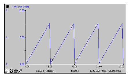
Weekly Cycle = Counter(1,8) produces a linearly increasing cycle which begins at 1, runs up to 8, and then repeats itself. The cycle thus translates simulation time into days of the week. Its behavior is shown in the following graph. In the example, From time has been set to 1.

The PULSE builtin generates a pulse input of a specified size (volume). When using the PULSE builtin, you have the option of setting the time at which the PULSE will first fire (first pulse), as well as the interval between subsequent PULSEs. Each time that it fires a pulse, the software pulses the specified volume over a period of one time step (DT). Thus, the instantaneous value taken on by the PULSE builtin is volume/DT. Volume can be either a variable or a constant. Specify the first pulse and interval values as constants.
If you don't provide a value for first pulse, the software generates the first pulse at the outset of your simulation run and continues to use it. This form is intended for situations where you have a quantity of material you want to put into a stock. If you don't provide an interval, the software generates subsequent pulses each DT of the model simulation (that is to say always). Setting interval to 0 yields a single pulse that doesn't repeat; it's the equivalent of specifying an interval that's greater than the length of the simulation.
Example:
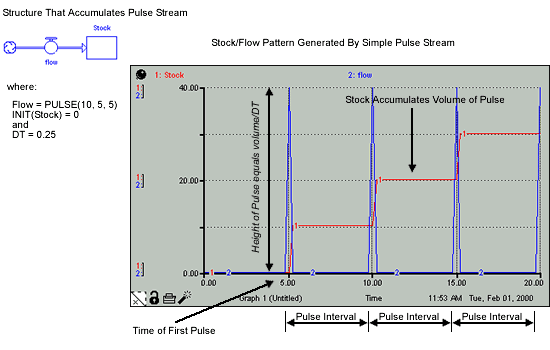
The following figure shows the structure, equations, and behavior pattern for a simple PULSE stream that accumulates in a stock.
The RAMP builtin generates a linearly increasing or decreasing input over time, with a specified slope. Optionally, you may set the start_time at which the ramp begins, and the end_time at which the ramp stops. The slope and time values can be either expressions or constants.
As the simulation progresses, RAMP returns a 0 before its time to begin has been reached. If you don't set RAMP's time, it will begin at the outset of the simulation.
Example:
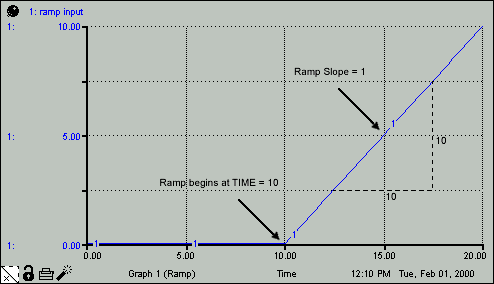
Ramp_Input = RAMP(1,10) generates the pattern shown in the following figure.
The SINWAVE builtin returns a time-dependent sine wave, with the specified amplitude and period. The SINWAVE builtin uses the absolute value of the amplitude you specify to generate the sine wave. To produce meaningful wave results, choose a DT that's significantly smaller than the period of the wave. A DT equal to a quarter of the period gives triangle waves. A smaller DT gives results which better approximate a continuous curve.
Examples:
SINWAVE(10,5) generates a sine wave with an amplitude of 10 units and a period of 5 time units.
SINWAVE(-5,2) generates a sine wave with an amplitude of 5 units and a period of 2 time units.
The STEP builtin generates a one-time step change of specified height, which occurs at a specified time. The height and time values can be either variables or constants.
If the optional <duration> is specified, the step will continue for that duration, then return to 0. Technically the step will be on the interval[<time>,<time>+<duration>). If <duration> is not specified the step will continue to the end of the simulation.
If the optional <interval> is specified (after <duration>) the step will repeat after the value of <interval> from when it returned to 0. This allows the creation of a repeated sequence of steps are regular intervals.
Example:
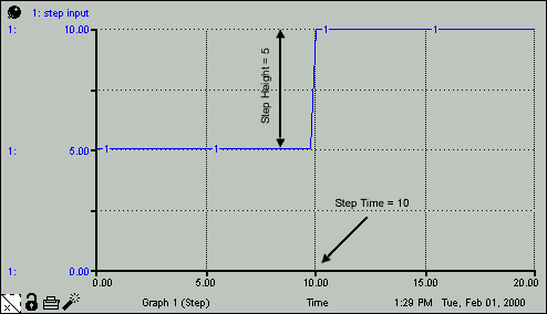
Step_Input = 5 + STEP(5,10) generates the behavior pattern shown in the following figure.
