Example:
EXPBOUND(1, 9, TIME, exponent, 2, 8)
The mathematical builtins perform mathematical operations on their input expressions, generating a result. Most commonly, you'll use the mathematical functions to define converters, which form the micro-logic of your model. Mathematical functions do a wide variety of operations, as detailed below.
This section describes the following builtins:
The ABS builtin returns the absolute value of expression. The expression value can be either a variable or a constant.
Example:
ABS(-1) equals 1
The EXP builtin gives e raised to the power of expression. The expression value can be either a variable or a constant. The base of the natural logarithm, e is also known as Euler's number; e is equal to 2.7182818... EXP is the inverse of the LN builtin (natural logarithm). To calculate powers of other bases, use the exponentiation operator (^).
Examples:
EXP(1) equals 2.7182818 (the value of Euler's constant)
EXP(LOGN(3)) equals 3
2^3 equals 8 (2 raised to the third power)
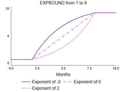
EXPBOUND(<yfrom>, <yto>, <x>, <exponent>, <xstart>, <xfinish> )
The EXPBOUND builtin transitions from yfrom when x is xstart to yto when x is xfinish following an exponential curve with the given exponent. If exponent is 0 the transition is linear, if it is negative the transition is fast near xstart and becomes slow near xfinish, and if it is positive the transition is slow near xstart then becomes fast near xfinish as shown below.
Example:
EXPBOUND(1, 9, TIME, exponent, 2, 8)
The INF builtin is equivalent to infinity (∞), and refers to something without any limit.
For example, you can define the capacity of a conveyor as unlimited by using the INF builtin.
The INT builtin gives the largest integer less than or equal to expression. The expression value can be either a variable or a constant.
Because of the internal calculations associated with the Runge-Kutta methods, the INT function may report non-integer values when you use the 2nd- or 4th-order Runge-Kutta computation methods. This is because reported values for flows are averaged across internally computed, but not reported, times.
Examples:
INT(8.9) equals 8
INT(-8.9) equals -9
The ISNAN returns 1 if the variable value is NAN, 0 otherwise. It is very useful when working with data or using the HISTORY builtin with other runs.
The LN builtin calculates the natural logarithm of expression. The expression value can be either a variable or a constant. Natural logarithms use Euler's constant, e, 2.7182818..., as a base. For LN to have meaningful results, expression must evaluate to a positive value. LN is the inverse of the EXP function, e raised to the power of expression.
Examples:
LN(2.7182818) equals 1
LN(EXP(3)) equals 3
LN(8)/LN(2) equals 3 (the base 2 logarithm of 8)
LN(-10) returns ? (undefined for non-positive numbers and will generate a divide by 0 error message)
The LOG10 builtin gives the base 10 logarithm of expression. The expression value can be either a variable or a constant. For LOG10 to be meaningful, expression must evaluate to a positive value. LOG10 is the inverse of the letter E in scientific notation, or base 10 exponentiation (10 raised to the power of expression).
Examples:
LOG10(10) equals 1
LOG10(1E5) equals 5
LOG10(8)/LOG10(2) equals 3 (the base 2 logarithm of 8)
LOG10(-10) returns ? (undefined for non-positive numbers and will generate a divide by 0 error)
LOGISTICBOUND(<yfrom>, <yto>, <x>, <xmiddle>, <speed>[, <xstart>[, <xfinish>]] )
The LOGISTICBOUND builtin transitions from yfrom when x is xstart to yto when x is xfinish following a logistic (s-shaped) curve with the given speed. If speed is less than or equal to 0 the transition is linear, it is slow near xstart and becomes fastest at xmiddle, and then slows approaching xfinish.
Example:
LOGISTICBOUND(1, 9, TIME, 5, 1, 1, 10)
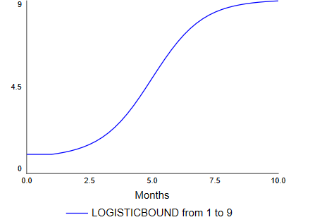
If xstart and xfinish are left off the transition is from -infinity to infinity, but practically does not look very different from the above example. Using the start and finish guarantees that the result will exactly match the specified yfrom and yto.
Note xstart and xfinish do not need to be symmetric around xmiddle. Depending on speed there may a noticeable corner at the transition point.
The MAX builtin gives the maximum value across the array if called with 1 argument, or between the two expressions if called with two arguments.
Example:
Purchases = MAX(0,Desired_Purchases) returns the larger value among Desired Purchases and 0. In this example, the MAX function will prevent Purchases from taking on negative values.
highest_temp = MAX(temp[*]) where temp is arrayed by location will find the temperature of the hottest location.
To report the maximum value across a subset of the dimensions of an arrayed input variable, specify an asterisk (*) to include all of the elements across a dimension.
Example:
Maximum Value for Salary = MAX(Salaries[*,*])
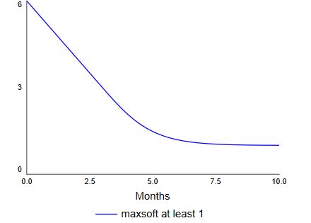
The MAXSOFT builtin returns a value that is never less than hard_minum and transitions from its input to hard_minimum smoothly. The value of tolerance determines how soon this transition from the input occurs. IF tolerance is 0 then MAXSOFT is the same as MAX.
Example:
MAXSOFT(6-TIME, 1, 2)
The MEAN builtin calculates the arithmetic mean across the elements in <array or expression> when called with 1 argument or across the arguments when called with more than one argument. The calculation is defined as the sum of the elements, divided by the number of elements in the array or the sum of the arguments divided by the number of arguments.
Examples:
Average Salary for Employees = MEAN(bobs_salary, marys_salary, franks_salary)
The MIN builtin gives the minimum value among the arrayed variables or expressions contained within parentheses.
Example:
Spending = MIN(Desired_Spending,Allowable_Spending) returns the smaller value among Desired Spending and Allowable Spending.
output = MIN(material[*]*factor_productivity[*]) will give output based on the most constraining input (Leonte
To report the minimum value across a subset of the dimensions of an arrayed input variable, specify an asterisk (*) to include all of the elements across a dimension.
Example:
Minimum Value for Salary = MIN(Salaries[*,*])
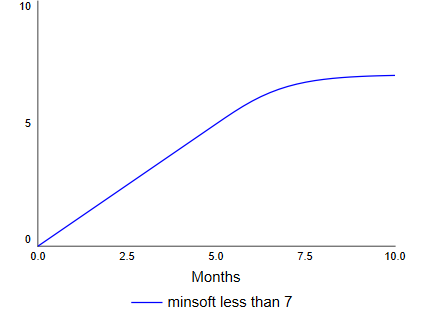
The MINSOFT builtin returns a value that is never larger than hard_maximum and transitions from its input to hard_maximum smoothly. The value of tolerance determines how soon this transition from the input occurs. IF tolerance is 0 then MINSOFT is the same as MIN
Example:
MINSOFT(TIME, 7, 2)
The MOD builtin calculates the remainder.
Examples:
x MOD y equals the remainder when the value of x is divided by the value of y
5 MOD 3 equals 2
The NAN builtin sets an invalid value for a variable (NAN stands for Not a Number). It is useful for controlling when a plot will appear on a graph. For example, to show values only between times 5 and 7 you could use
var = IF TIME < 7 or TIME > 5 THEN NAN ELSE other_var
Care should be taken not to use a variable with value NAN in an equation as this will normally result in a divide by zero error.
You can also use NAN with arguments (as in NAN(Converter_1,Converter_2)). This is useful to provide equations for variables that are not expected to be computed. This equation format is included automatically when working in The CLD Window.
The ROOTN builtin returns the order root of expression. The expression value can be either any expression, and the order value can be an expression or constant. If the order is not an integer it will be rounded to an integer. For meaningful results, expression must be greater than or equal to 0 when order is even. If order is 0 ROOTN returns 1. Negative orders are treated as 0.
Examples:
ROOTN(144,2) returns 12
ROOTN(4,2.3) return 2 (2.3 is rounded to 2)
ROOTN(-27,3) returns -3
ROOTN(-27,2) returns ? (undefined for negative numbers and will generate a divide by 0 error)
NoteROOTN(a,b) will return the same value as a^(1/b) when a is positive and b is a positive integer.
Note If order is a constant then the units of the expression will also have their root taken for units checking.
The ROUND builtin rounds expression to its nearest integer value.
Because of the internal calculations associated with the Runge-Kutta methods, the ROUND builtin doesn't always return integer values when you use the 2nd- or 4th-order Runge-Kutta computation methods. When your model constructs rely on the ROUND builtin, be sure to use Euler's method.
Examples:
ROUND(9.4) equals 9
ROUND(9.64) equals 10
The SAFEDIV builtin allows you to divide two things without first checking that the denominator in the expression is nonzero. It returns numerator/denominator as long as result of that computation is allowed and finite. If denominator is 0, or extremely close to 0, it will return 0, or, if onzero has been specified, it will return onzero. SAFEDIV can be used to prevent divide by zero messages stopping the simulation, and to allow other model values to be computed reasonably.
Examples:
SAFEDIV(10,5) returns 2
SAFEDIV(1,0) returns 0
SAVEDIV(1,1E-150,1E9) returns 1E150
SAFEDIV(1E150,1E-150,1E9) returns 1E9
Note You can use // as a shortcut for SAFEDIV with a//b the same as SAFEDIV(a,b)
The SQRT builtin gives the square root of expression. The expression value can be either a variable or a constant. For meaningful results, expression must be greater than or equal to 0.
Examples:
SQRT(144) returns 12
SQRT(-242) returns ? (undefined for negative numbers and will generate a divide by 0 error)