The miscellaneous builtins are designed to be used in a variety of different circumstances. You'll find them helpful in setting up specific scenarios for a model simulation (COUNTER, CGROWTH, RUNCOUNT, SENSIRUNCOUNT), in doing simple trend analysis and extrapolation (FORCST, TREND), for simplifying computation in project models (REWORK), and in reusing or defining data sets for graphical functions (LOOKUP). Together, the miscellaneous functions offer a wealth of capabilities which can fill out the details of your model.
This section describes the following builtins:
In many instances, you'll want a stock to grow in compounding fashion, at a certain percentage rate per unit of time. You'd like to input the percentage growth rate, and to have the results of the process be independent of the DT that's being used in the model simulation.
The CGROWTH function enables you to define such DT-independent growth rates. Simply provide CGROWTH with a per-period percentage growth rate. When embedded in a compounding process, CGROWTH will ensure that the stock grows at the per-period rate you've specified, independent of the DT that's being used.
Example:
Growth Fraction = CGROWTH(10) produces 10% per unit time compound growth for the stock illustrated below. The specific numerical results of this compound growth process will be independent of the DT being used for the simulation.
Returns the current system clock time on the computer the software is running on. The time is the number of seconds since midnight, January 1, 1970 (often referred to as epoch time). Generally, this function is most useful for published simulations for which data are being collected. See Data Collection for more discussion and ways to convert this value to a recognizable date and time.
Activities in a simulation model are often driven by external cycles. A financial department, for example, runs on a 30-day billing cycle. A business concern may have seasonal demand cycles. When the simulation is meant to run over several cycles, it's useful to know where in the cycle you are, at any point in time.
The COUNTER builtin enables you to define such time-dependent cycles. You provide COUNTER with starting and ending values for the cycle. COUNTER will map start to the From time you've specified in the Run Specs dialog box. It will subsequently return linearly increasing values, as time progresses. Once COUNTER has counted up to the end, it will reset itself to start and begin the cycle anew.
Example:
Weekly Cycle = Counter(1,8) produces a linearly increasing cycle which begins at 1, runs up to 8, and then repeats itself. The cycle thus translates simulation time into days of the week. Its behavior is shown in the following graph. In the example, From time has been set to 1.
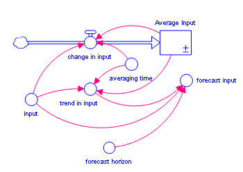
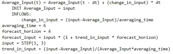
The FORCST builtin performs simple trend extrapolation. FORCST calculates the trend in input, based upon the value of input, the first order exponential average of input, and the averaging time. (Think of the averaging time as the time over which you want to calculate a trend.) Then FORCST extrapolates the trend into the future; you specify the distance into the future, by providing a value for horizon. If you don't specify an initial value initial, FORCST substitutes 0 for the initial value of the trend in input.
The FORCST builtin is equivalent to the structural diagram and equations shown in the following figure.
Example:
Sales_Forecast = FORCST(Sales,10,15,0) produces a forecast of sales 15 time units into the future. The forecast is based on current sales, and the trend in sales over the last 10 time units. The initial growth trend in sales is set to 0.
Tip: If you encounter noise in the variable to be forecasted, you may wish to filter the randomness by basing your forecast on an exponential smooth of the variable. To do this, use the SMTH1 or the SMTH3 function (described later in this section).
The INF builtin is equivalent to infinity (∞), and refers to something without any limit.
For example, you can define the capacity of a conveyor as unlimited by using the INF builtin.
The LOOKUP builtin evaluates the <graphical variable> at the given <expression> (versus using the equation stored in the graphical function itself). This function uses the interpolation model (Continuous, Extrapolated or Discrete) specified in the graphical.
The LOOKUPAREA builtin returns the area under the <graphical variable> for all values up to and including the given <expression>. For example, a graphical that is constant at 1 will have an area given by the input less the first x value in the graphical. This is a convenient function for normalizing the output of graphical. The interpolation mode of the graphical is ignored in this function.
For continuous and stepwise graphicals LOOKUPAREA will return 0 when expression is less than the first x point and the total area under the curve when it is greater.
For extrapolated graphicals the area at the first point in the graphical is treated as 0, and when called with a smaller number it will return the negative of the area between that point and the first x point. This allows you to use LOOKUPAREA(g,x1)-LOOKUPAREA(g,x2) to give the area under the graphical between x1 and x2 even when one (or both) of them are above or below the x axis of the graphical itself.
The LOOKUPINV builtin reverses the normal lookup logic returning the x value in the <graphical variable> that would generate the given <expression> as output. As long as the graphical is monotonic (the y value getting bigger for each successive x value, or the y value getting smaller for each successive x value) it will return a value. If the graphical is marked as Extrapolated it will use extrapolation to compute a value, otherwise it will return the first or last point when out of range.
If a graphical is not monotonic (including starting of stopping with a flat spot), the first x value to generate the y value will be returned. If there y value is out of range then NAN will be returned.
The LOOKUPMEAN builtin finds the mean value of X from the beginning of the first x value of <graphical variable>until the value of <expression>. The mean is computed by treating the graph from the beginning to expression as a probability density function (pdf). Most commonly, LOOKUPMEAN will be used on a distribution with the x axis ranging from 0 to 1 evaluated at 1. This is very helpful when using the graphical as a delay profile distribution for a conveyor. For example:
delay_profile ((0,0),(0.5,1),(0.8,0.01),(0.1,0))
average_delay = 8
maximum_delay=INIT(average_delay/LOOKUPMEAN(delay_profile,1)
The conveyor would then use maximum_delay as the transit time, and the inflow would use delay_profile as the profile.
Note The above equations require that the graphical be defined on the range 0 to 1, otherwise the max value will be distorted and the mean transit time through the conveyor will not be average_delay.
The LOOPSCORE builtin returns the relative contribution of a loop to determining behavior at each time in the simulation. See Loops That MatterTM Overview for discussion and references.
The arguments <var1>, <var2> and so on must define a feedback loop. If they do not, LOOPSCORE will return NAN at all times.
LOOPSCORE is added automatically when you create Loop variable from the Loops Panel. Typically, this is the only way it is used, so you won't ever add it by hand. Like a Summing Converter, a Loop Score variable does not have any connectors going in. Unlike a Summing Converter, however, you can't use a Loop Score variable in the equation of another variable. This is because Loops Scores are not computed until after a simulation finishes, and thus the value returns is always NAN during the simulation. For this reason the variable will also not animate on a graph during simulation, but only display afterward.
You can change a Loop Score variable to a Pathway Score variable. This will change the LOOPSCORE builtin to the PATHSCORE builtin, and also add the first <var> at the end to close the path.
The MLPANN builtin allows you to create a Multi-Layer Perceptron Artificial Neural Net. This is useful for approximating functional relationships using trained neural nets, where the training is done using the optimizer.
<input> is a vector of inputs to be passed through the neural net.
<shapes> is a vector of values that describes the topology of the neural net. The number of elements in it determines the number of layers in the network, and the value of each element the number of nodes in each layer.
<weights> is a vector of values that specifies the weight to be given to the incoming connection to each node (on all layers). The total number of weights must be equal to the product of the elements of the <shapes> vector. The weights are typically included as part of an optimization to train the neural net.
<biases> is a vector of values that scale the input to each of the nodes. It can be a vector of 1s, but must have the same number of elements as <weights>.
<activation_type> specified the type of activation function used. A value of 1 will use a tanh activation function (most common), 2 a sigmoid activation function, and 3 a non-negative activation function (negative values treated as 0) function. Any other value will use a linear activation function (no attenuation).
The NAN builtin sets an invalid value for a variable (NAN stands for Not a Number). It is useful for controlling when a plot will appear on a graph. For example, to show values only between times 5 and 7 you could use
var = IF TIME < 7 or TIME > 5 THEN NAN ELSE other_var
Care should be taken not to use a variable with value NAN in an equation as this will normally result in a divide by zero error.
You can also use NAN with arguments (as in NAN(Converter_1,Converter_2)). This is useful to provide equations for variables that are not expected to be computed. This equation format is included automatically when working in The CLD Window.
PATHSCORE(<var1>, <var2>, ...)
The PATHSCORE builtin returns the product of the raw (unnormalized) Link Scores along a path of connected variables. See Loops That MatterTM Overview for discussion and references.
The arguments <var1>, <var2> and so on must be on a path (that is <var1> must be a cause of <var2> and so on. If are not, PATHSCORE will return NAN at all times.
When PATHSCORE is called with two variables it returns link score. While PATHSCORE can be used in any equation, it will be automatically input into the equation for a Pathway Score variable. You can create a Pathway Score variable from a Loop Score variable by changing its type. This sill add the first entry last in order to close the loop. You can also create a Loop Score variable from a Pathway Score variable - this will remove that last variable since the Loops assumes closure.
In many instances, you'll want to represent a rework process. In the following figure, for example, a production process is used to draw down a work backlog. A portion of the work (defectives) is shunted back to an earlier stage in the process to be reworked.
In the following figure, a conveyor represents an inspection activity. The leakage flow from the activity moves rejected material to an earlier stage in the process, where it will subsequently be re-worked.
In either situation, using a simple fraction to represent the rework percentage will overstate the cumulative flow of material through the rework process. Each time that material passes through the inspection activity or production process, a fraction of it will be sent back to be re-worked. Double-counting can ensue. For example, if 100 units are sent through the process initially, a 10% defective fraction would send 10 units back to be re-worked in the first round. In the second round, 1 unit (10% of the 10 units) would be sent back. And so on. After the fact, more material than 10% has been re-worked! In most cases, this isn't what you intended.
To get around this double-counting phenomenon, the software provides the REWORK builtin. Use it only to represent a rework flow which deposits material at a point somewhere upstream in the main chain. Simply specify the percentage of total work flow that you want to flow back upstream to be reworked. The percentage value should be a value between 0 and 100.
Notes: When using a draining process to represent
the rework flow, the REWORK builtin is not an appropriate choice.
When the defective flow goes to a cloud, double-counting is not an issue.
Hence, REWORK isn't required.
Example:
The previous figure shows the results of using REWORK(10) to define the leakage fraction for the leakage flow from "Inspection Activity". With a total of 100 units of material entering the system through the "entering wip" flow, a total of 10 units of work flow through the "failing inspection" flow, over the course of the simulation.
The RUNCOUNT builtin returns the number of complete runs prior to the current run.
When you create a new model or open an existing model and run it for the first time, RUNCOUNT equals 0 (that is, the number of runs prior to the current run equals 0).
When you run the model a second time, RUNCOUNT equals 1.
This is useful when you're building an interactive interface for your model and you want some change to take place after a few runs (for example, turn on a piece of structure).
The SENSIRUNCOUNT builtin returns the number of the run in a sequence of sensitivity runs, or 0 if the current run is not part of a set of sensitivity runs.
When you start a sensitivity run SENSIRUNCOUNT will return 1, then 2, then 3 and so on up to the total number of runs being made. Each time you start a new sensitivity run, this sequence will repeat. This can be useful if you want to do something different for specific sensitivity runs. For example, using NORMAL(100,10,SENSIRUNCOUNT) would return a different random number sequence for each run in sensitivity. This value will be independent of the other sensitivity parameters and invariant across sensitivity executions.
The TREND builtin calculates the trend in input, based on the value of input, the first order exponential average of input, and the exponential averaging time averaging time. TREND is expressed as the fractional change in input per unit time. If you don't specify an initial value initial, TREND substitutes the value 0 for the initial value of the trend.
The TREND builtin is equivalent to the structural diagram and equations shown in the following figure.
Example:
Yearly_Change_in_GNP = TREND(GNP,1,.04)
This equation calculates the annual change in the input GNP. It starts with an initial value of .04 (4% per year).