 stock = dt * flow
By far the simplest algorithm used by the software is Euler's method. In this method, the computed values for flows provide the estimate for the change in corresponding stocks over the interval DT. In the simple cooling model, the initialization and iteration phases look like this:
Step 1. Create a list of all stocks, flows and converters in required order of evaluation.
Step 2. Calculate initial values of all stocks, flows and converters (in order of evaluation).
Time = From Time
--->Time = 0
Stockt=0 = f(initial values, stocks, converters, flows)
--->INIT Temperature = 100
Converters = f(stocks, converters, flows)
--->constant = 0.5
Flows = f(stocks, converters, flows)
--->cooling = Temperature * constant
Step 1. Estimate change in stocks over the interval DT.
Calculate new value for Stocks based on this estimate.
Stockt = Stockt-dt +
--->Temperature = Temperature + (-cooling) * dt
Step 2. Calculate new values for flows and converters (in order of evaluation).
Converters = f(stocks, converters, flows)
--->constant = 0.5
Flows = f(stocks, converters, flows)
--->cooling = Temperature * constant
Step 3. Update simulation time. Stop iteration when Time >= simulation stoptime.
Time = Time + dt
The numeric output generated by the cooling model, for the first four time units, is shown in the following table. The output was produced using Euler's method, with DT = 0.5, beginning balances, and summed reporting of flows.
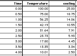
As the data show, cooling declines in proportion to Temperature. The data set for Temperature approximates an exponential decay pattern, such as the one shown in How model equations are solved.
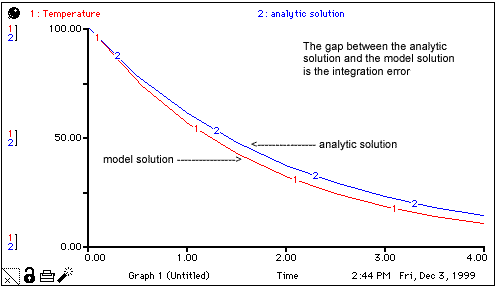
At this point, however, it is useful to ask about the accuracy of this approximation. As the following graph shows, the model output is not very accurate when compared with the analytical solution to the equivalent equation (Temperature = 100e-0.5*time). Because Euler's method simply uses the value calculated for the flow as its estimate for the change in the stock over the interval DT, and because the interval is a large one (relative to the continuous case), an integration error is introduced. This integration error is the difference between the two curves on the plot.
 See Also