The miscellaneous builtins are designed to be used in a variety of different circumstances. You will find them helpful in setting up specific scenarios for a model simulation (COUNTER), in doing simple trend analysis and extrapolation (FORCST, TREND), in establishing relationships which require knowledge of the simulation specs or of specific model entities (CGROWTH, REWORK, RUNCOUNT), and in reusing or defining data sets for graphical functions (LOOKUP). Together, the miscellaneous functions offer a wealth of capabilities which can fill out the details of your model.
This section describes the following builtins:
In many instances, you will want a stock to grow in compounding fashion, at a certain percentage rate per unit of time. You'd like to input the percentage growth rate, and to have the results of the process be independent of the DT which is being used in the model simulation.
The CGROWTH function enables you to define such DT-independent growth rates. Simply provide CGROWTH with a per-period percentage growth rate. When embedded in a compounding process, CGROWTH will ensure that the stock grows at the per-period rate you have specified, independent of the DT which is being used.
Example:
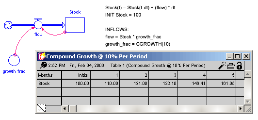
Growth Fraction = CGROWTH(10) produces 10% per unit time compound growth for the stock illustrated below. The specific numerical results of this compound growth process will be independent of the DT being used for the simulation.

Activities in a simulation model often are driven by external cycles. A financial department, for example, runs on a 30-day billing cycle. A business concern may have seasonal demand cycles. When the simulation is to run over several cycles, it is useful to know where in the cycle you are, at any point in time.
The COUNTER builtin enables you to define such time-dependent cycles. You provide COUNTER with starting and ending values for the cycle. COUNTER will map start to the From time you have specified in the Run Specs dialog box. It will subsequently return linearly increasing values, as time progresses. Once COUNTER has counted up to the end, it will reset itself to start and begin the cycle anew.
Example:
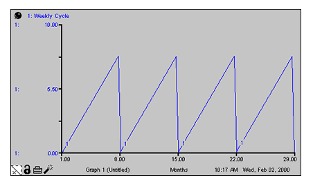
Weekly Cycle = Counter(1,8) produces a linearly increasing cycle which begins at 1, runs up to 8, and then repeats itself. The cycle thus translates simulation time into days of the week. Its behavior is shown in the following graph. In the example, From time has been set to 1.
The FORCST builtin performs simple trend extrapolation. FORCST calculates the trend in input, based upon the value of input, the first order exponential average of input, and the averaging time. (Think of the averaging time as the time over which you wish to calculate a trend.) Then FORCST extrapolates the trend into the future; you specify the distance into the future by providing a value for horizon. If you do not specify an initial value, FORCST substitutes 0 for the initial value of the trend in input.
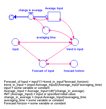
The FORCST builtin is equivalent to the structural diagram and equations shown in the following figure.
Example:
Sales_Forecast = FORCST(Sales,10,15,0) produces a forecast of sales 15 time units into the future. The forecast is based on current sales, and the trend in sales over the last 10 time units. The initial growth trend in sales is set to 0.
Tip: If you encounter noise in the variable to be forecasted, you may wish to filter the randomness by basing your forecast on an exponential smooth of the variable. To do this, use the SMTH1 or the SMTH3 function (described later in this section).
The INF builtin is equivalent to infinity (∞) and refers to something without any limit.
For example, you can define the capacity of a conveyor as limitless by using the INF builtin.
The LOOKUP builtin evaluates the <graphical variable> at the given <expression> (versus using the equation stored in the graphical function itself).
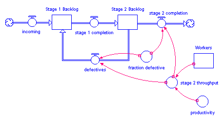
In many instances, you will want to represent a rework process. In the following figure, for example, a production process is used to draw down a work backlog. A portion of the work (defectives) is shunted back to an earlier stage in the process to be reworked.
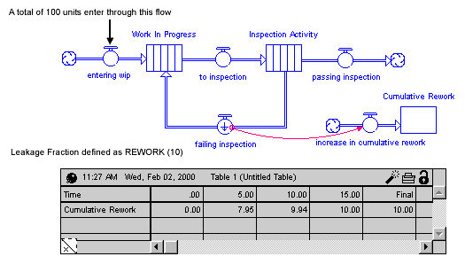
In the following figure, a conveyor represents an inspection activity. The leakage flow from the activity moves rejected material to an earlier stage in the process, where it will subsequently be re-worked.
In either situation, using a simple fraction to represent the rework percentage will overstate the cumulative flow of material through the rework process. Each time that material passes through the inspection activity or production process, a fraction of it will be sent back to be re-worked. Double-counting can ensue. For example, if 100 units are sent through the process initially, a 10% defective fraction would send 10 units back to be re-worked in the first round. In the second round, 1 unit (10% of the 10 units) would be sent back. And, so on. After the fact, more material than 10% has been re-worked! In most cases, this is not what you intended.
To get around this double-counting phenomenon, the software provides the REWORK builtin. Use it only to represent a rework flow which deposits material at a point somewhere upstream in the main chain. Simply specify the percentage of total work flow that you desire to flow back upstream, to be reworked. The percentage value should be a value between 0 and 100.
Notes: When using a draining process to represent
the rework flow, the REWORK builtin is not an appropriate choice.
When the defectives flow goes to a cloud, double-counting is not an issue.
Hence, REWORK is not required.
Example:
The previous figure shows the results of using REWORK(10) to define the leakage fraction for the leakage flow from the Inspection Activity. With a total of 100 units of material entering the system through the entering wip flow, a total of 10 units of work flow through the failing inspection flow, over the course of the simulation.
The RUNCOUNT builtin returns the number of complete runs prior to the current run.
When you create a new model or open an existing model and run it for the first time, RUNCOUNT equals 0 (that is, the number of runs prior to the current run equals 0).
When you run the model a second time, RUNCOUNT equals 1.
This is useful when you are building an interactive interface for your model
and you want some change to take place after a few runs (for example, turn on
a piece of structure
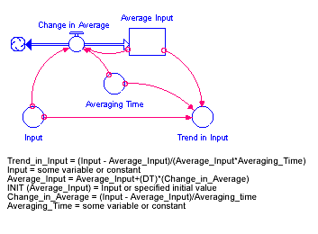
The TREND builtin calculates the trend in input, based upon the value of input, the first order exponential average of input, and the exponential averaging time averaging time. TREND is expressed as the fractional change in input per unit time. If you do not specify an initial value, TREND substitutes the value 0 for the initial value of the trend.
The TREND builtin is equivalent to the structural diagram and equations shown in Figure 7-28.
Example:
Yearly_Change_in_GNP = TREND(GNP,1,.04)
This equation calculates the annual change in the input GNP. It starts with an initial value of .04 (4% per year).
