This section describes the following builtins:
Present value (pv), future value (fv), periodic payment (pmt), number of periods (nper), and interest rate per period (rate) are standard financial parameters in cash flow problems involving constant payments. The FV, PMT, and PV builtins calculate future value, periodic payment, and present value based upon the values of the other financial parameters.
Use the following cash flow conventions in depicting PV, FV, and PMT: cash received is represented by a positive number, cash paid out is represented by a negative number. See the example below for an illustration. Note that rate and nper must refer to the same period. For example, if nper is the number of months, then rate must be the effective monthly interest rate. Finally, for each of the financial builtins, the first payment is assumed to occur at the end of the first period.
The software uses the following equations to solve for one financial argument in terms of the others:
pv * (1 + rate)nper + (pmt / rate) * ((1 + rate)nper -1) + fv = 0
(for rate <> 0)
pv + pmt * nper + fv = 0
(for rate = 0)
Example:
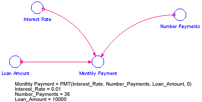
You received an automobile loan of $10,000, at an effective monthly interest rate of 1%. You must repay the loan in 36 monthly payments made at the end of each month. What are your monthly payments?
Your structural diagram, and the corresponding equations, are shown in the following figure.
The software returns the value for Monthly Payment as -332.14, indicating that the payment is an expense.

The NPV function calculates the net present value of a stream of input, using a discount rate of rate; rate refers to the effective per-period discount rate for your model simulation. The value returned by NPV is the present value (at the outset of your simulation run) of the stream of inputs from model start time to a given simulation time. You may specify an optional initial value initialfor the calculation; otherwise, the initial value of input serves as the initial value.
The NPV function, when used in a converter, will produce the same results as the stock in the structure and equations shown below. The discount factor is normalized to the Time Specs setting for start time, so that the initial condition of the denominator evaluates to a value of 1.

change_in_NPV = input * discount_factor
discount_factor = 1/(1 + rate)^(TIME - STARTTIME + DT)
input = constant or variable
rate = constant or variable
INIT Net_Present_Value = constant
Examples:
Net_Present_Value = NPV(10, .05) generates the pattern shown in the following graph. The values for Net Present Value represent the present value - at time 0 - of the constant stream of benefits, given the effective per-period discount rate of 5%.
